About a year and a half ago, I posted a tutorial on Excel’s vlookup() function. This remains one of my favorite data manipulation tools because of how you can use it to combine information from multiple sources.
But sometimes, you already have all the information you need; it’s just, well, messy. The most common scenario is this: you request some data, and in response, someone gives you a list. The only problem is that the list isn’t broken up the way you expected. Perhaps you really need a person’s street address, city, and ZIP code in separate columns, but you were given a spreadsheet where they’re all combined into one. Or maybe you weren’t given a spreadsheet at all. Perhaps it was just several rows of information pasted into an email.
This actually happened to me a few weeks ago. I sent the names of a couple dozen students to our school’s representative at the company who takes portraits for us, and I asked if she could send back the appointment details for each of those students. I was hoping to use this information to send out reminder emails via a mail merge.
Unfortunately, what I received back was not the nicely formatted table I was hoping for. Instead, it was this:
- Celeste Bateman 1/19/22 8:45am P9H5WLVS
- Aditya Jensen 1/19/22 9:00am XF27AHR7
- Dione John 1/19/22 9:15am ZVYT6C9B
- Eshaan Morrow 1/19/22 9:15am YY2BF9L9
- Sultan Livingston 1/19/22 9:15am 5XJ7CZ35
- Lilly Grace McCarty 1/19/22 9:30am GLL3ZHVR
- Bo Singh 1/19/22 9:30am GQMAPK7G
- Zaara Lee Sims 1/19/22 9:45am CU5MT99K
- Meadow Lozano 1/19/22 9:45am RQAS6N3E
- Daniella Joyce 1/19/22 10:00am L47Q2JUS
- Reuben Edmonds 1/19/2022 10:45am W2KHGWTP
- Hilary Ventura 1/19/22 10:45am DK8JSYJ5
- Ilyas Wheatley 1/19/22 10:45am 3RZ4MLP4
- Aasiyah Hail 1/19/2021 12:00pm 9GF2S3G9
- Sakina Cartwright 1/19/22 12:00pm 9A5LU5LD
- Jasper Cabrera 1/19/22 12:15pm W2QEY8LL
(Names and appointment codes have, of course, been changed to protect people’s privacy. And technically, what I was sent wasn’t even a bulleted list. I did that to make it look nicer on this page.)
This was all useful information, but without the names, dates, times, and appointment codes separated into their own columns, I would have no way of automatically looking up the ID numbers and parent email addresses that I would need for sending reminders. I also wouldn’t be able to put the different pieces of information into separate fields in my email template.
Fortunately, Excel has a tool for just this type of problem: Text to Columns.
Objective
Our goal is to convert several rows of “messy” data into a clean spreadsheet with separate columns for each piece of information.
Materials
All we’ll be using today is Microsoft Excel. (Note: You can use these same techniques with Google Sheets. The tools are just in different places.)
For the messiest of data sets, additional tools and plugins may be necessary. For now, the goal is to master the basics. With that in mind, this tutorial will cover the Text to Columns function itself and how to use Find/Replace to make life a little bit easier when that isn’t enough.
Part 1: Predictable Data
Let’s start by assuming the data you’re working with is relatively predictable. What I mean by this is the information is always in the same order and it is always divided up the same way.
Take a look at the list below:
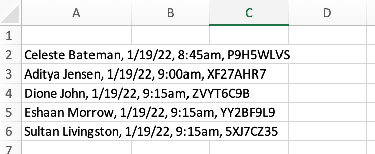
- Celeste Bateman, 1/19/22, 8:45am, P9H5WLVS
- Aditya Jensen, 1/19/22, 9:00am, XF27AHR7
- Dione John, 1/19/22, 9:15am, ZVYT6C9B
- Eshaan Morrow, 1/19/22, 9:15am, YY2BF9L9
- Sultan Livingston, 1/19/22, 9:15am, 5XJ7CZ35
In this example, the data always follows the same order: Name, Date, Time, Code. On top of that, each piece of information is always separated by a comma.
Here’s how we’d turn that into an Excel spreadsheet.
Step 1: Paste In the Data
The first part is kind of obvious. Start by opening up Microsoft Excel. Then, select the list above and copy it to the clipboard. Next, select the first cell in the second row (i.e. cell B1) and paste in the data. It should look something like this:
Before we move on, it’s a good idea to give that column a heading. I’ve found that Text to Columns can do weird things if the first row is empty. Let’s just call it Data.

Step 2: Split Up the Data
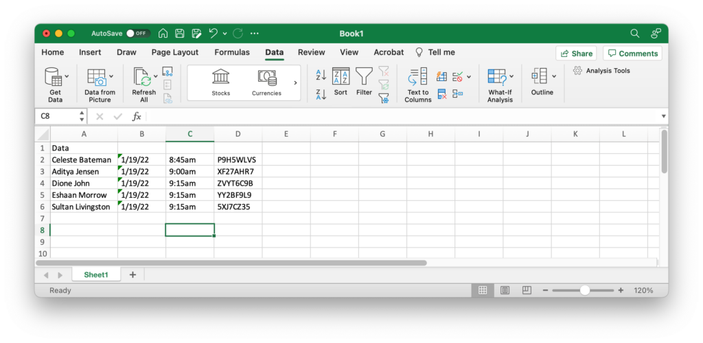
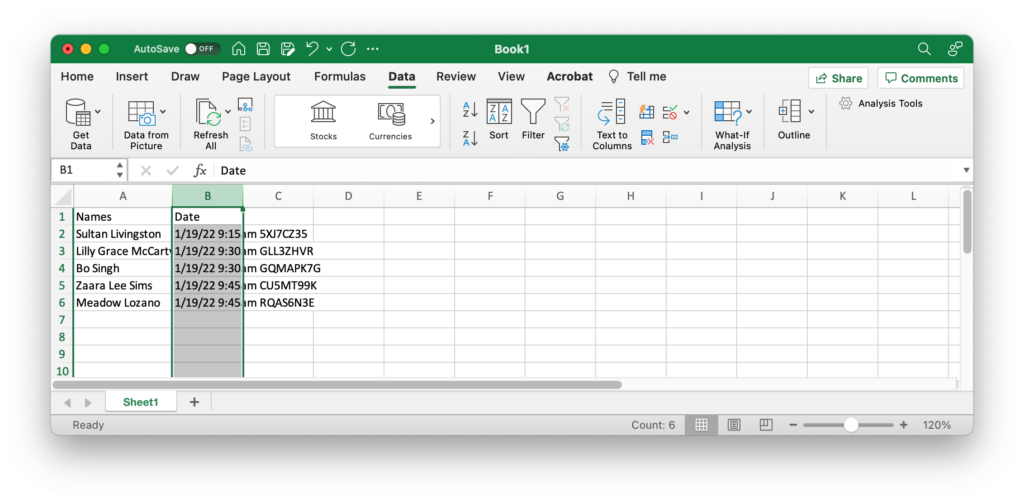
Now, click the heading for Column A to select all the information.

Next, find the Data tab in the toolbar above your spreadsheet. (Technically, Microsoft calls this toolbar the “Ribbon.”) In that tab, there should be an option called Text to Columns. Depending on your version of Excel, whether you’re using a Mac or PC, and how wide your window is, the size, location, or appearance of this button may vary. But in some form or another, it should be there. I’ve circled it toward the right in the screenshot below.
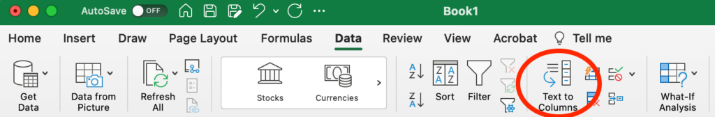
If you haven’t already, go ahead and click that button.
This pops up a somewhat intimidating dialog box with ugly looking previews and multiple steps to work through. Oh joy!
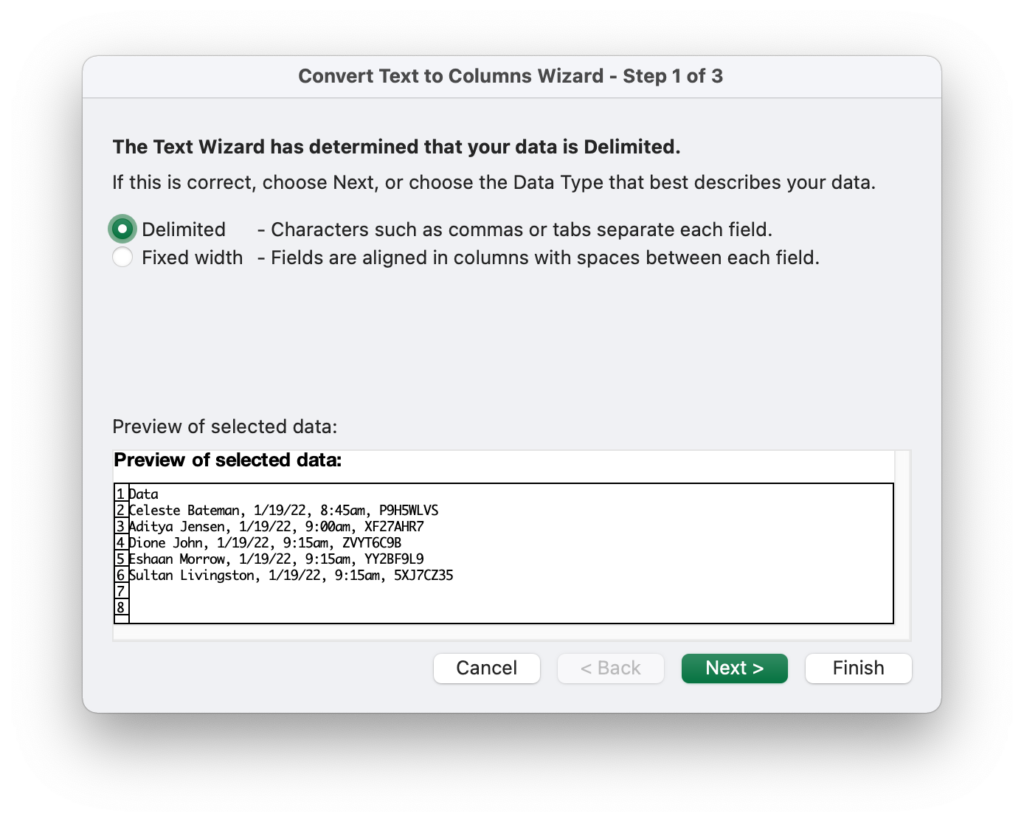
But it’s actually not so bad. For this first step, the vast majority of the time, you want to use the first option: delimited. This means that some symbol—be it a comma, tab, or even a blank space—separates each piece of data.
(You only want to use fixed width in the rare situation where there is no obvious separator character and every piece of information is the exact same size in each row.)
Make sure delimited is selected, and click Next.
Now, you should see something like this:
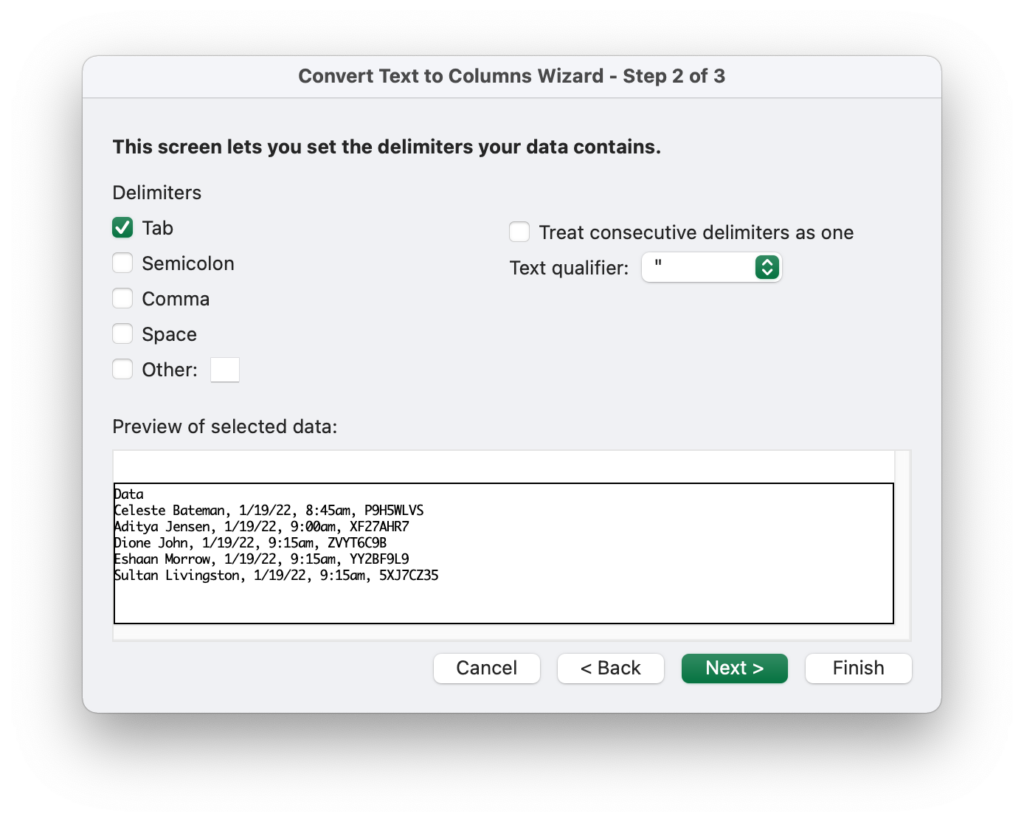
This page is asking us to choose which character is being used as the delimiter (i.e. the separator). In this case, we’re using a comma, so make sure to check that box and uncheck all the others. When you’re done, it should look like this:
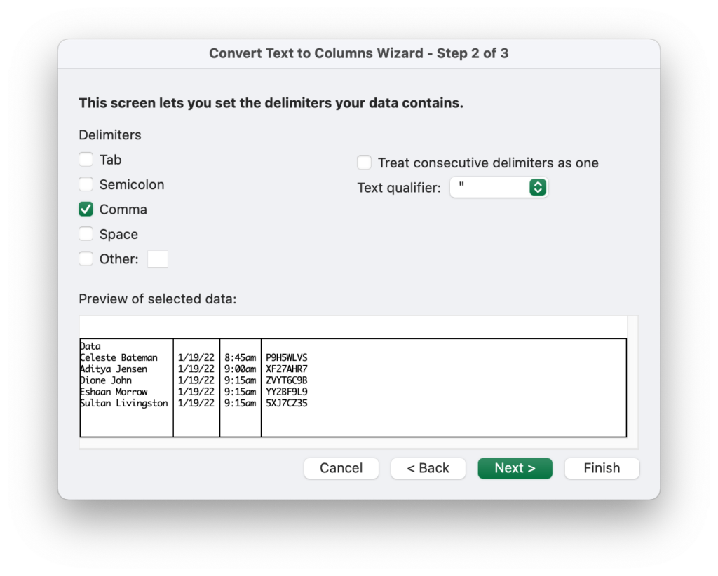
Notice that Excel has added column markers to the preview to show us what the results will look like. This looks pretty good, so go ahead and click Next.
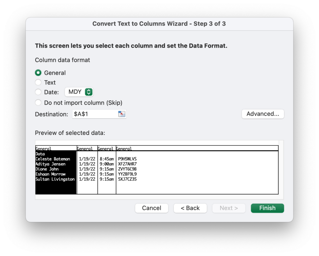
This final page of the dialog box lets you set up data formats for each piece of information. We don’t need to do anything with that for this tutorial, but if you know what you’re doing, and it’s applicable to your paritcular data set, this can be a helpful step. For now, we’re going to skip it. So just click Finish.
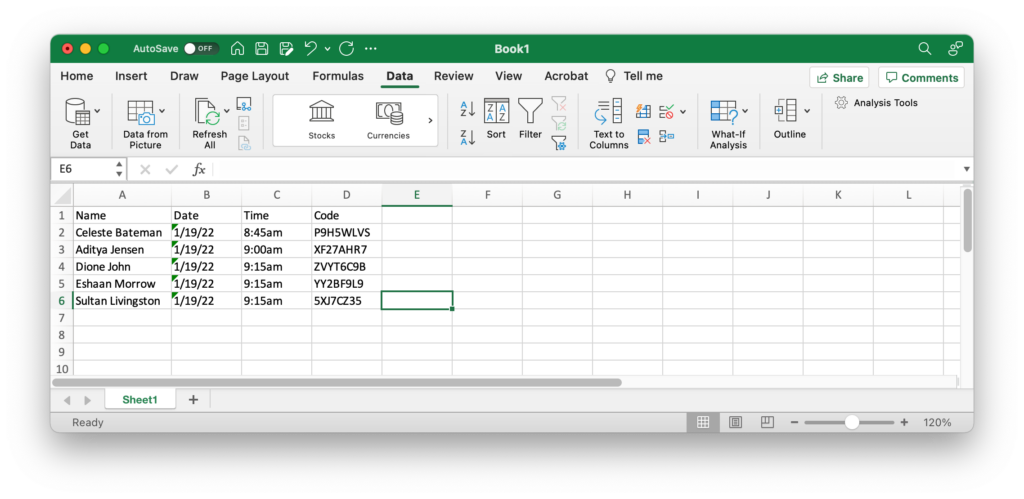
You should now see something like this:
Step 3: Clean It Up
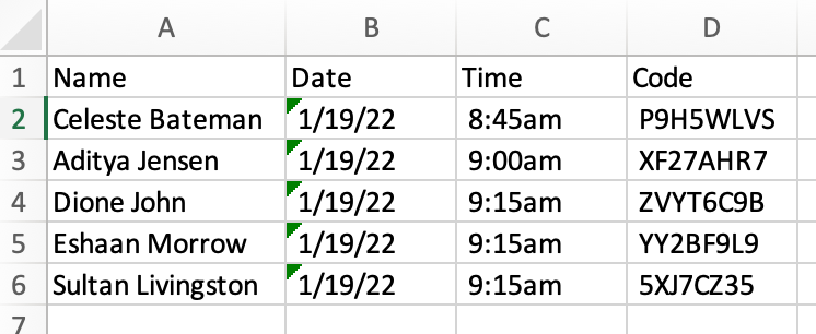
Now that we’ve broken up the data, we can do a little work to make it prettier. The first thing you’ll almost always want to do is add some headings for all the new columns.
If you’re lucky (when working with a real data set), you may be done at this point. However, that is often not the case. For example, there’s something slightly weird about our sample data. If you look closely, you’ll notice that there’s an extra space at the beginning of each column. This is because the original data had a space after each comma (e.g. Celeste Bateman, 1/19/22, 8:45am, P9H5WLVS).
Depending on what we want to do with this data, that might not matter. But I’m a perfectionist, so I’m going to do a little more cleanup. We can easily remove those spaces by using Excel’s trim() function.
First, we add a new column. The easiest way to do this is to right-click on a column heading (e.g. Column C) and choose Insert.
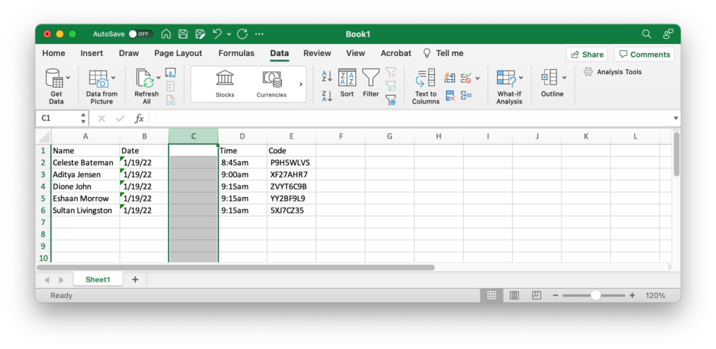
Now, type the following formula into cell C2: =trim(B2)
Press the enter key and you should now see a date in Column C, but without the extra space.
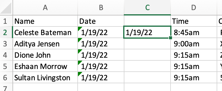
Now, make sure that new date is selected, and double-click the little square in the bottom-right corner of the cell. Excel should now automatically apply the trim() function to the entire column.

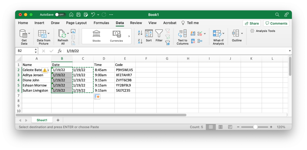
Now, while that information is still selected, paste it to the clipboard. Then, highlight the original column like so:
Next, right-click on the selected cells and find the option in the menu to paste values. Now you’ll see this:
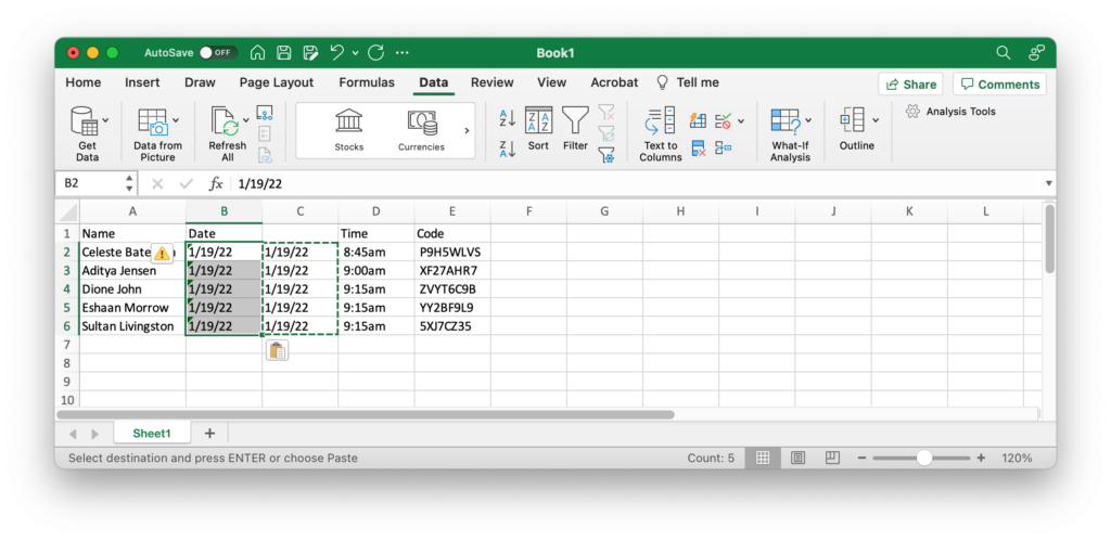
If this worked correctly, you should now be able to delete Column C and repeat the process for the remaining columns. If all goes well, you should now have a clean set of data with everything in its own column and no extra spaces!
Pro Tip: What if your original data already has multiple columns?
Suppose your original data was already in the form of a table or spreadsheet but you still need to split up one of the original columns (or maybe even a few of them). In this case, the process is pretty much the same, but there’s one important caveat…
When you split up a column, Excel will overwrite the data in adjacent columns! So make sure to insert as many blank columns as you expect you’ll need need between the column you’re splitting up and the one to its right.
Part 2: Messier Data
In the previous example, I made things easy by putting some commas between the fields that needed splitting. But data in real life is not always so clean.
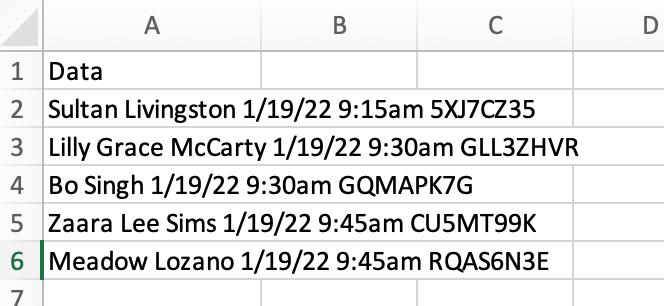
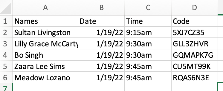
You may recall that there weren’t actually any commas in the list I received from the photo company. Rather than make you scroll all the way back to the top of this page, here are a few of those entries again:
- Sultan Livingston 1/19/22 9:15am 5XJ7CZ35
- Lilly Grace McCarty 1/19/22 9:30am GLL3ZHVR
- Bo Singh 1/19/22 9:30am GQMAPK7G
- Zaara Lee Sims 1/19/22 9:45am CU5MT99K
- Meadow Lozano 1/19/22 9:45am RQAS6N3E
The only thing separating each field in this data set is a blank space, but here’s what happens if I try to use that as the delimiter character when doing Text to Columns:
Here are the same results in table form, just to make it more clear:
| Sultan | Livingston | 1/19/22 | 9:15am | 5XJ7CZ35 | |
| Lilly | Grace | McCarty | 1/19/22 | 9:30am | GLL3ZHVR |
| Bo | Singh | 1/19/22 | 9:30am | GQMAPK7G | |
| Zaara | Lee | Sims | 1/19/22 | 9:45am | CU5MT99K |
| Meadow | Lozano | 1/19/22 | 9:45am | RQAS6N3E |
As you can see, the columns don’t line up correctly. The third column is a mix of names and dates; the fourth is a mix of dates and times. And we even ended up with an unexpected sixth column.
The problem is that not every space in the original set of data is actually a delimiter. Take a look at rows two and four: Lilly Grace McCarty and Zaara Lee Sims both have two-part first names; the space is actually part of their name. That’s what threw off the data, and this is the exact sort of thing that makes a “messy” data set messy.
For a data set this small, it’s not such a big deal to go back and fix it manually, but what if we were working with, say, 100 names?
Read on for a neat little trick I’ve found for dealing with this sort of thing. It won’t work in all cases, but it’s definitely a life-saver when it does!
Step 1: Look for a Pattern
So the issue is that we need to break up a bunch of data separated by spaces but we don’t want to separate the individual names. What would make this operation a lot easier would be if there were some other separator—say, a semicolon or comma—after the names. Then, we could use that as the delimiter.
So let’s just add one in!
But remember, I hate doing things by hand if I don’t have to, so let’s find a way to automate this. If you look carefully at the bulleted list, you’ll see that each name is followed by the same exact series of characters: 1/. (To clarify: that’s a space, followed by a number 1 and a slash.) Significantly, this pattern does not appear anywhere else in the data, which means we can use it as a definitive way to identify where names always end and dates always begin!
Step 2: Use Find/Replace to Add In a Delimiter
Now that we’ve identified a pattern, we can use that pattern to add in our own delimiter. To do this, we use the Find and Replace tool.
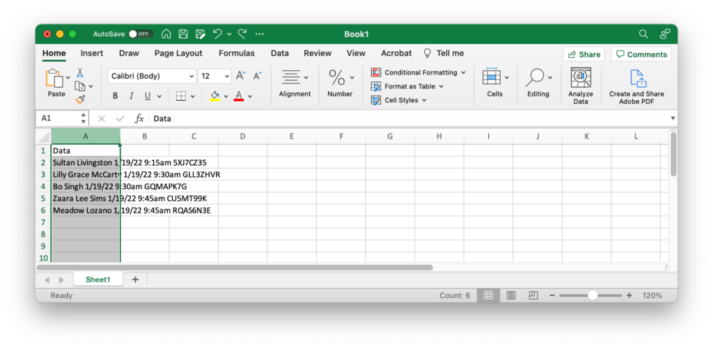
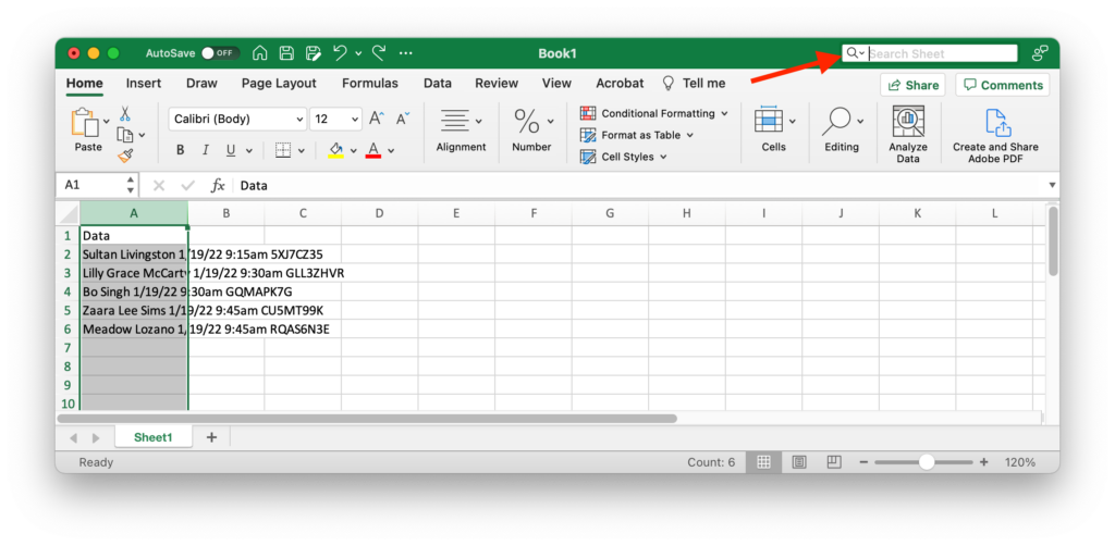
First, if you haven’t done so already, go ahead and paste the new data set into Excel. (Don’t forget to put a heading—i.e. “Data”—in the first row.)
Now, make sure the appropriate column is selected.
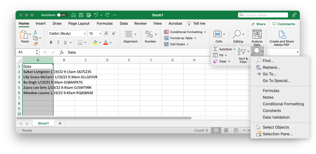
Next, find the Find/Replace tool. There are several ways to access this. On my version of Excel, I can click the magnifying glass in the toolbar to open a search box. Then, I click on another little magnifying glass, which opens a drop-down menu containing the Replace… command.
Alternatively, I can also find the Replace… command by going to the Home tab in the toolbar and then clicking on Find and Select. If you don’t see this option, you may need to first click on Editing. (Excel’s constantly changing toolbar is one of the app’s more annoying behaviors if you’re trying to help someone find a particular feature.)
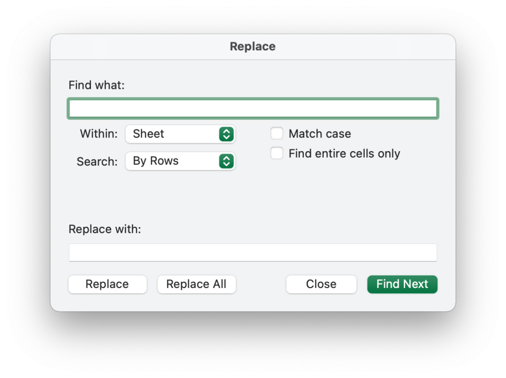
Once you’ve found the Replace… command (wherever it might be hiding), go ahead and click on it. You’ll see the following dialog box:
Now, underneath “Find what,” we need to put in that pattern we noticed: 1/. (Don’t forget the space at the beginning.)
Then, underneath “Replace with,” we’re going to use that same pattern, but we’ll replace the space with a semicolon: ;1/.
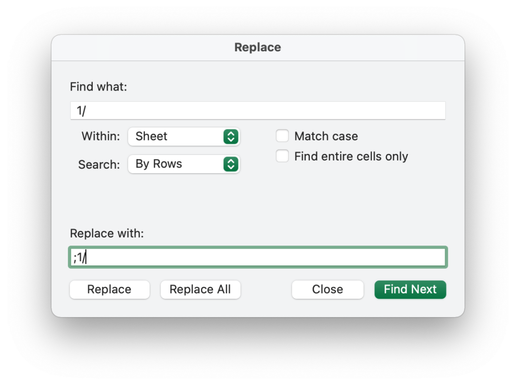
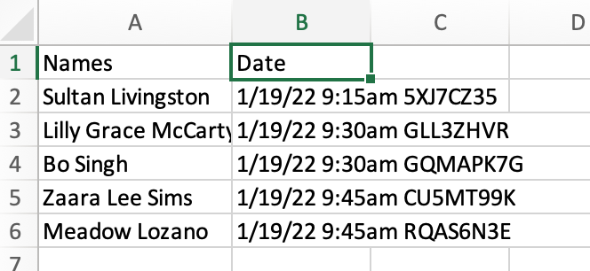
If your dialog box looks like the screenshot above, go ahead and click the Replace All button. (Don’t be tempted by that highlighted, enticing button in the corner…) An alert should pop up telling you that several replacements have been made. You can clear that alert and close the dialog box. Your data should now look like this:

Notice that there is now a semicolon between each name and date.
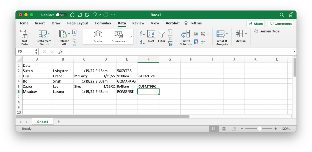
The next step is to select the first column again and use the Text to Columns tool like we did before. But this time, let’s tell it that the delimiter is a semicolon instead of a space.
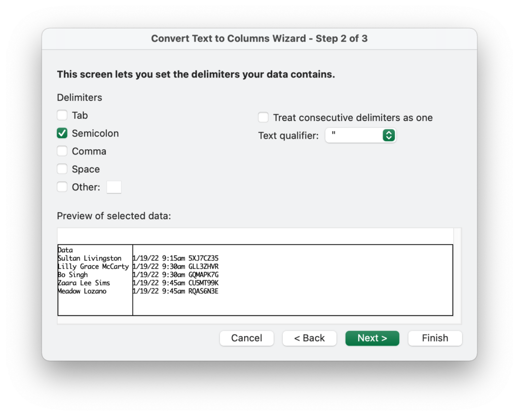
As you can see from the screenshot above, this will not split up all the columns for us, but it will separate the names from everything else, and that’s good enough for now!
Step 3: Repeat (If Necessary)
Now we need to figure out if there are any more spots in our data that need extra care to separate. The good news is that in this example, there aren’t any. Everything else is very cleanly separated by a single blank space. If that wasn’t the case, we might have needed to do some more find/replace operations.
Step 4: Separate the Rest of the Columns
Before we move on, lets add in some updated column headings.
Now, we can select Column B…
…and perform another Text to Columns operation. This time, we’ll go back to using a space as the delimiter.

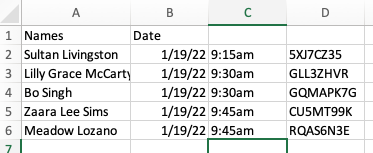
As you can see, the rest of our columns should get divided up as expected, resulting in this:
The final step is to add in our new column headings.
Wrapping Up
The combination of Find/Replace and Text to Columns can go a long way to making messy data sets easier to work with.
Keep in mind that sometimes you might need to do a Find/Replace operation more than once on a single column to add in the delimiters, especially if there isn’t just one pattern to look out for.
And sometimes the data is so messy, that even Find/Replace isn’t enough. When that happens, I like to export the spreadsheet to a CSV file, open it in a fancy text editor, and use an advanced technique called “Regular Expressions” to look for more complicated patterns. But that’s a blog post for another day!