Okay. I’m about to dedicate an entire blog post to my all-time favorite spreadsheet function.
Not only did this function truly open my eyes to the hidden power of Microsoft Excel; it was also my gateway drug to the wider world of relational databases.
I’m talking about vlookup().
Imagine you have multiple tables of information, each serving a particular purpose, but one day, you need to somehow splice these tables together.
For example, suppose you run an online store. Somewhere in your operation there is probably a list of all your customers along with their contact information, the date they registered for an account, and perhaps some demographic details. Suppose you also happen to have a record of all your sales for the past year. This table could include things like the name of the product that was purchased, the date of the transaction, and the customer who bought it.
Now, imagine your boss wants you to do some research. “I want you to find out more about our customers,” she says. “I want to know whether people who registered accounts a few years ago are still active buyers on our site.” Later on, your boss comes by again and asks you to send a marketing email to those folks thanking them for their loyalty.
So what do you do?
Remember that your sales data is in one list and your registration dates and contact info are in a completely different list. You could switch back and forth between these lists, copying and pasting the information from one to another. Done!
Okay, but what if you have hundreds of customers? Copying and pasting that information individually would take a long time. Alright, in that case, couldn’t you just copy an entire column from one table into the other? Well, actually, no. It turns out you sold thousands of items that year. Not every customer necessarily bought an item. And some customers may have had multiple transactions! These two data tables do not have a one-to-one match.
So now what?
Well, what you need is a way to look up data from one table based on the information in another. As it turns out, this is exactly what vlookup() does. The vlookup() function takes a value from one table (e.g. the buyer of a product in the sales list), looks for it in another table (e.g. the list of accounts), and then returns a value from another column in that second table (e.g. the registration date or email address). In other words, it does exactly what you’re doing when you copy and paste from one table to another, but it does it for you! This might not seem like a big deal for a single row, but if you can do this for all 1000+ rows at once, that’s a lot of saved time!
Sound exciting to you? Here’s my step-by-step tutorial on how it’s done.
Materials
To learn how to execute a vlookup(), you need a copy of Microsoft Excel and two sets of data that have at least one column in common. To help you out, I’ve created a sample spreadsheet to work with.
For the purposes of this tutorial, both sets of data are saved to that single file, but one of the cool things about vlookup() is that it will even work across multiple files!
I’ll be using the Windows version of Excel for this tutorial, but it works just as well in macOS. The vlookup() function also works pretty much identically in Google Sheets!
Step 1: Look At Your Data
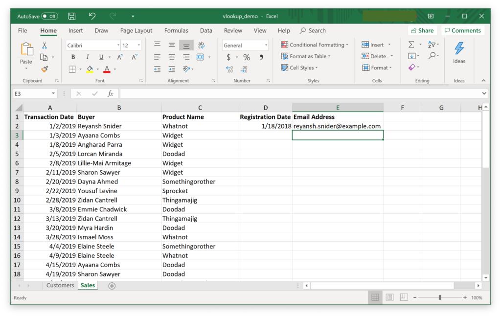
The first thing you need to do is get all the data you need to work with, so go ahead and open the sample spreadsheet. You’ll notice that I’ve broken it up into two tabs: Customers and Sales. This theoretical online store has 20 total customers and handled 50 transactions in 2019.
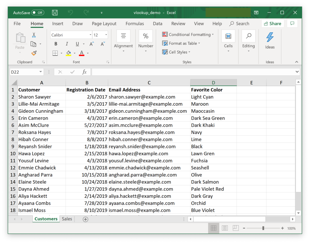
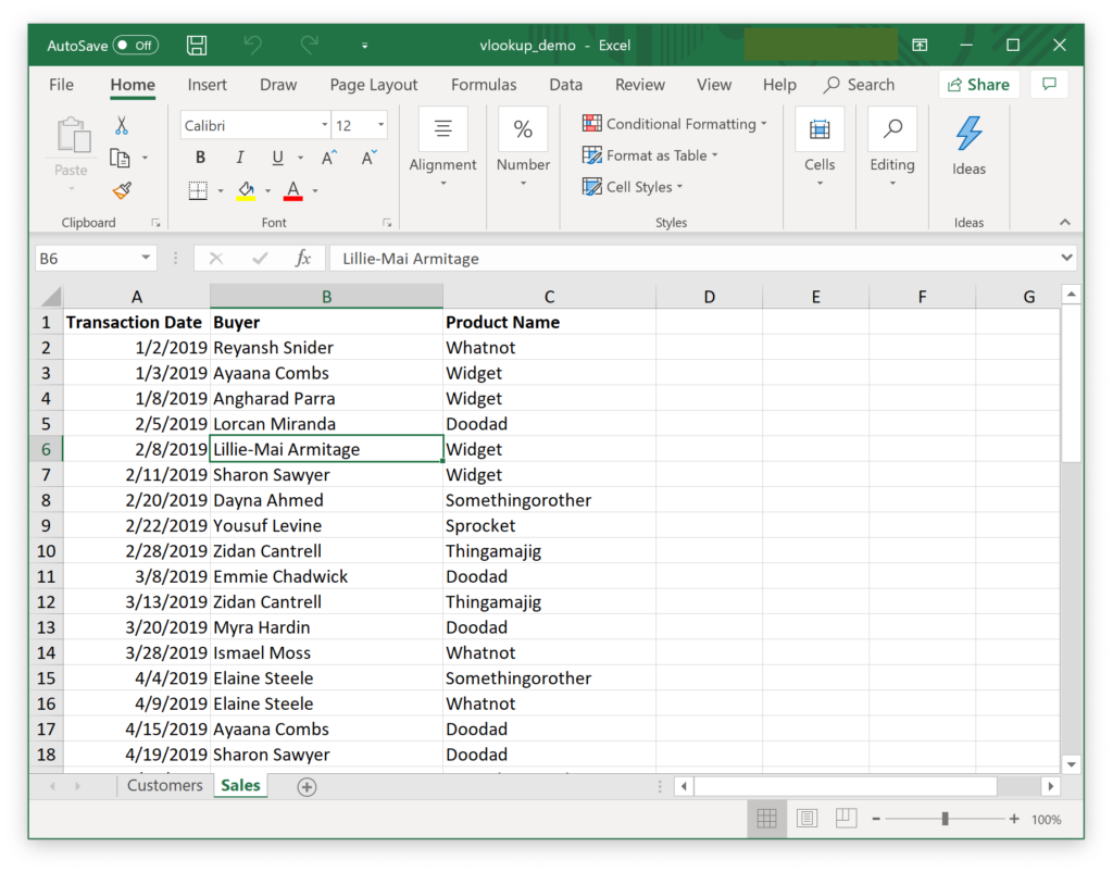
In order to combine the data, you need to figure out what piece of information they each have in common. In this case, you should notice that each table has a column containing people’s names. On the one tab, they’re called customers, and on the other tab they’re called buyers, but these actually represent the same people. That’s how the two tables are related, so you’re going to want to use those names as your lookup values.
Step 2: Add Some Columns for Your Lookup Data
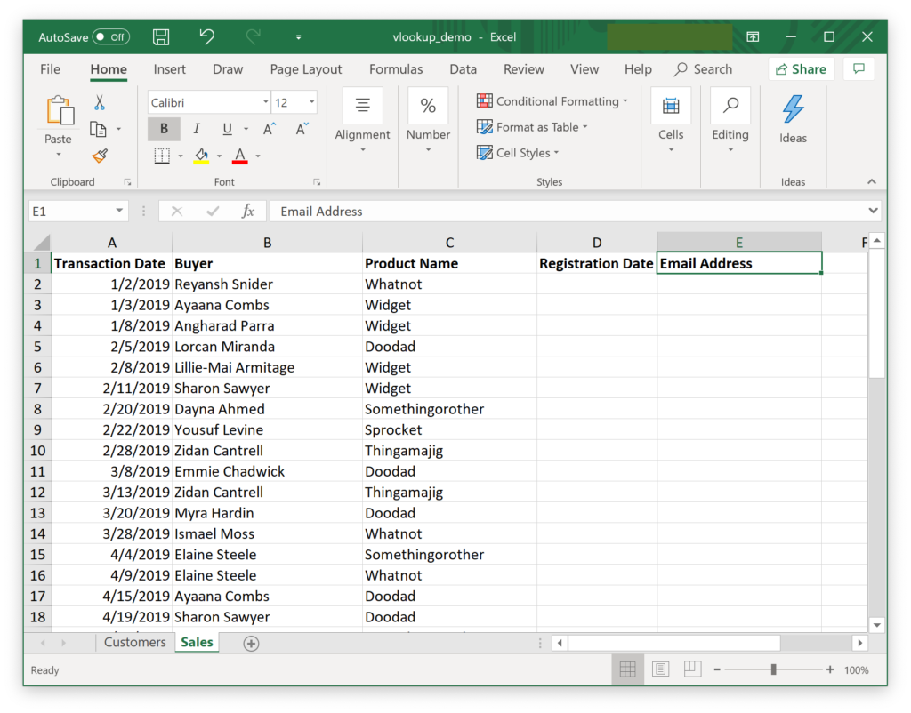
If you go back to our original scenario, you’ll recall that you have two goals: find out when this year’s buyers registered their accounts and determine their email addresses. So let’s add two new columns to the Sales tab to hold that information.
Step 3: Create Your Formulas
Overview of a VLOOKUP
Now that you have your new columns, you need to write a couple Excel formulas that use the vlookup() function to look up the values from the Customers tab.
Here’s how Excel defines the structure of the vlookup() function:
VLOOKUP(lookup_value, table_array, col_index_num, range_lookup)And here’s what that all means:
- VLOOKUP: That’s the name of the function.
- lookup_value: That’s the thing in the current table whose match we want to find in the other table.
- table_array: That’s the other table that we’re going to look in to find the matching value.
- col_index_num: That tells Excel which column contains the value you want to copy into the current table from the other table.
- range_lookup: That controls whether Excel looks for an exact or approximate match. (I’ll explain this further in a bit.)
Formula #1
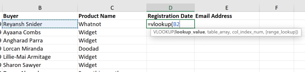
To write your formula, start by clicking in the first empty cell in the “Registration Date” column (i.e. D2). Then type in =vlookup(.
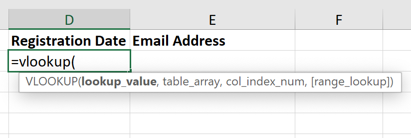
As you can see in the screenshot above, Excel pops up a helpful guide to remind you what to put in each part of the function.
The first thing we need is our lookup value. You can either type in B2, which is the cell representing our first buyer, Reyansh Snider, or you can click on this person’s name. (If you click, the B2 will be entered in automatically.)
Next, type in a comma so that Excel knows you’re moving on to the next input.
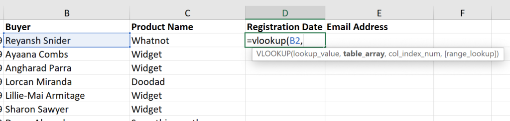
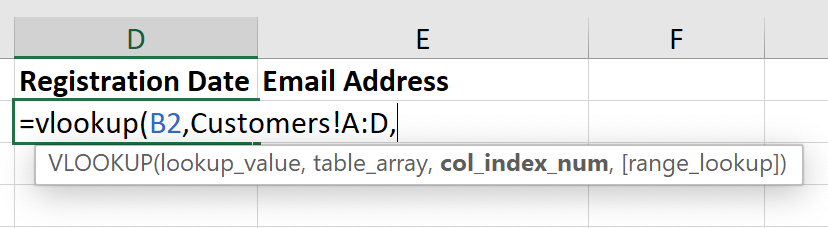
You’ll see that table_array is now highlighted. What we need to do here is provide a code (what Excel calls a range) that tells the function to look at the Customers table. In this case, the code we’re looking for is Customers!A:D. Huh? Let’s break it down:
- Customers! = Look inside the Customers tab.
- A:D = Look at columns A through D.
Once again, you can either type that code in directly…
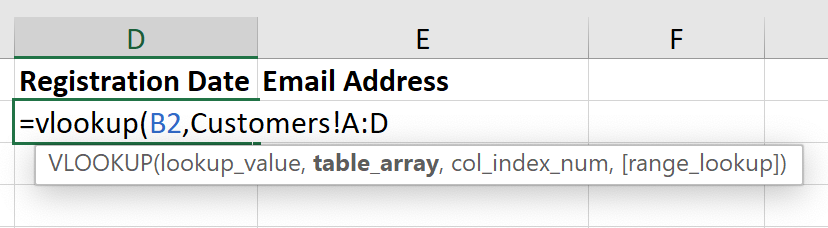
…or you can click to the other tab and highlight the columns you’re looking for to let Excel do it for you:
Whichever method you choose, be sure to follow it with a comma!
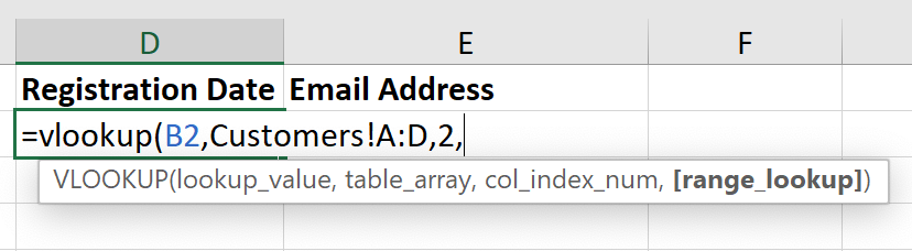
Now, you’r ready to put in your column number. But let’s take a step back for a second. The way the vlookup() function works is to look for your desired value in the very first column of the specified range. It always looks in the first column; there’s no way to change that. However, you can control which value it returns.
In the case of our example, you’re looking for looking for the registration date, which happens to be the second column in our range. (Column 1 is the name, and Column 2 is the registration date.) So the next piece of your formula is simply the number 2. (And of course, don’t forget the comma.)
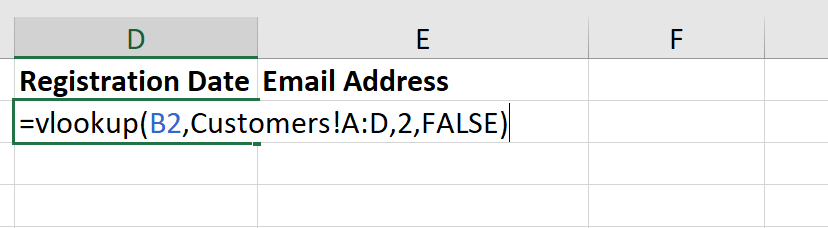
Now the slightly weird part. For this last parameter (“range_lookup”), we need to enter FALSE. This tells Excel to find an exact match. In other words, whatever the lookup value is, Excel should look for that and only that.
Once you type in FALSE, you can close the parenthesis. The vlookup() is complete!
In case you’re curious, if you were to put in TRUE (or leave it out altogether), Excel would look for an approximate match. The problem with approximate matches is that they only work for values that are properly sorted (i.e. numerically or alphabetically), but more importantly, it would make no sense for us to pick a customer whose name was only kind of like the one we’re looking for. I pretty much always use FALSE when I’m creating a vlookup.
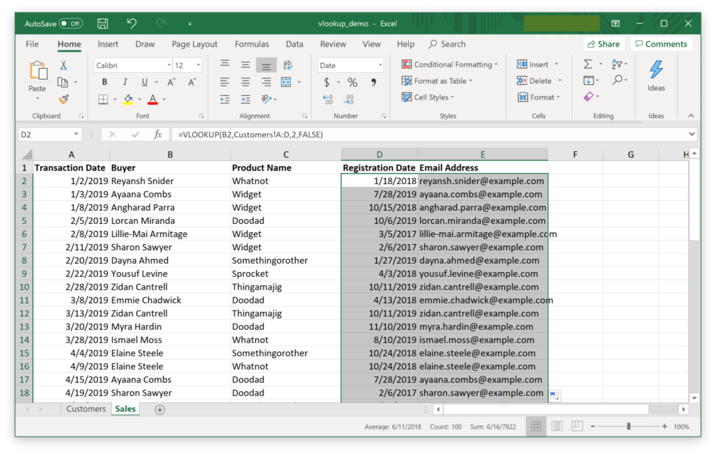
So anyway, your completed formula should now look like this:
=vlookup(B2,Customers!A:D,2,FALSE)You can go ahead and press the Enter key now.
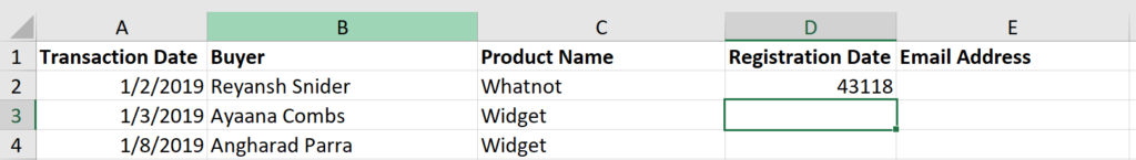
Wait, what the heck is 43118? Alas, this is just a quirky aspect of how Excel handles dates. You can easily fix this by highlighting column D, clicking the drop-down list in the “Number” section of the toolbar, and choosing “Short Date.”
Here’s an animation to help you out:
Formula #2
To look up this person’s email address, click into Cell E2 and create that same formula again. However, this time, use the number 3 where it asks for the column number:
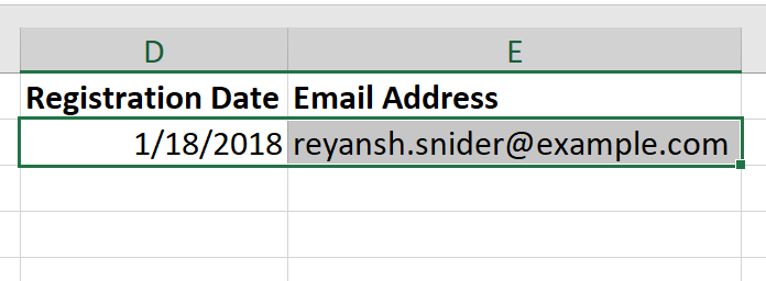
=vlookup(B2,Customers!A:D,3,FALSE)Assuming the formula was entered in correctly, you’ll now see an email address in Cell E2.
Step 4: Use the Auto-Fill
So now you’ve got the registration date and email address for the first buyer. Of course, that’s not enough. You actually want that information for every customer. Thankfully, there’s no need to type in the formula 96 more times. Instead, you can use Excel’s auto-fill feature.
The first step is to highlight these two cells.
Then look for the little green square in the bottom-right corner of the highlight box. (I’ve circled it in red below.)
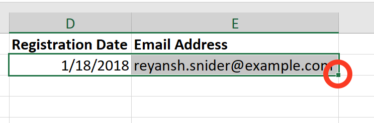
Now, all you have to do is hover over that square with your cursor so that it turns into a big plus sign.
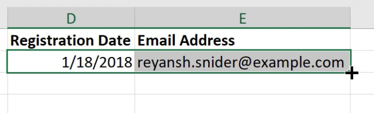
And then, just double-click. Excel will fill in all of the remaining dates and email addresses!
Step 5: Analyze Your Data
You have everything you need now to answer your hypothetical boss’s question. For instance, you can use Excel’s sorting features to organize this list by registration date. This might give you a sense of how many items were bought by “old” vs. “new” customers.
You could even use Excel’s “Remove Duplicates” feature so that each customer only appears in the list once. Now, you have a definitive list of only the customers who purchased items this year, conveniently sorted by registration date. This will make it easy to figure out who the most loyal customers are; plus, you’ve got all their email addresses right there!
I’ll leave it as an exercise to the reader to play with the sorting and “Remove Duplicates” features. If you’re unfamiliar with them, you’ll find them in the Data tab on the toolbar.
Wrapping Up
As I mentioned earlier, vlookup() can be used within a single file or across multiple files. You can even use it with multiple tables of data on a single tab.
In fact, there’s no rule that says you must set an entire table or spreadsheet as your lookup range.
In our example, we selected an entire spreadsheet, but you can also limit the range to just a portion of the sheet by typing in something like this as your range: $A$2:$E$7. That tells Excel to use A1 as the top left corner of the table and E7 as the bottom right. Meanwhile, the dollar signs tell Excel to use that same range for every row when you do the auto-fill.
When you’re ready to get super-fancy, you can use Excel’s filtering tools, pivot tables, and other functions to divide up, summarize, and reformat your data in all sorts of ways. I hope to cover some of these tools in future blog posts!
Finally, I’d like to give a shout-out to the random name generator, random date generator, and random color generator that were used to create the sample spreadsheet for this tutorial.